Note

📥 Download this tutorial

Variability classification for a single brown dwarf spectrum

Classify a brown dwarf spectrum as a candidate variable or non-variable using the NIR spectral-index variability scheme implemented in seda.classify_variability.

This tutorial shows how to:

• read an input spectrum,

• run the variability classification for either an L or T dwarf scheme,

• inspect the output stored in the VariabilityResult object,

• and optionally generate diagnostic plots of the index bandpasses and the index–index variability diagrams.

import seda
from seda.variability import classify_variability
import numpy as np
import os
from astropy.io import ascii
from numpy.typing import ArrayLike
from typing import Tuple, Literal, Optional, Union, Dict, List, Mapping
from matplotlib import Path

Read the spectrum of interest

As an example, let us read a near-infrared brown dwarf spectrum. You can replace this file by your own spectrum, as long as it contains wavelength and flux columns.

# path to the seda package
#path_seda = os.path.dirname(os.path.dirname(seda.__file__))

#spec_name = path_seda + '/docs/notebooks/data/0439-nirspec-Ldwarf.txt'
spec_name = '/Users/arrecifecosmico/seda/docs/notebooks/data/0439-nirspec-Ldwarf.txt'
spec = np.loadtxt(spec_name, comments='#').T

wave = spec[0]   # wavelength in microns
flux = spec[1]   # flux

If your input file contains uncertainties, you can still use them for your own bookkeeping, but the variability module currently requires only wavelength and flux arrays.

Explore the function documentation

As for other SEDA functions, you can inspect the function description directly in the notebook:

help(classify_variabilty)

Help on module seda.variability in seda:

NAME
    seda.variability

CLASSES
    builtins.object
        VariabilityResult

    class VariabilityResult(builtins.object)
     |  VariabilityResult(spectral_type: str, scheme: str, is_candidate_variable: bool, n_regions_triggered: int, n_regions_total: int, threshold: int, indices: Dict[str, float], regions_triggered: List[str], normalize: Optional[bool] = None) -> None
     |
     |  VariabilityResult(spectral_type: str, scheme: str, is_candidate_variable: bool, n_regions_triggered: int, n_regions_total: int, threshold: int, indices: Dict[str, float], regions_triggered: List[str], normalize: Optional[bool] = None)
     |
     |  Methods defined here:
     |
     |  __eq__(self, other)
     |
     |  __init__(self, spectral_type: str, scheme: str, is_candidate_variable: bool, n_regions_triggered: int, n_regions_total: int, threshold: int, indices: Dict[str, float], regions_triggered: List[str], normalize: Optional[bool] = None) -> None
     |
     |  __repr__(self)
     |
     |  summary(self) -> str
     |
     |  ----------------------------------------------------------------------
     |  Data descriptors defined here:
     |
     |  __dict__
     |      dictionary for instance variables (if defined)
     |
     |  __weakref__
     |      list of weak references to the object (if defined)
     |
     |  ----------------------------------------------------------------------
     |  Data and other attributes defined here:
     |
     |  __annotations__ = {'indices': typing.Dict[str, float], 'is_candidate_v...
     |
     |  __dataclass_fields__ = {'indices': Field(name='indices',type=typing.Di...
     |
     |  __dataclass_params__ = _DataclassParams(init=True,repr=True,eq=True,or...
     |
     |  __hash__ = None
     |
     |  normalize = None

FUNCTIONS
    classify_variability(wavelength, flux, *, spectral_type: str, normalize: bool = True, scheme: Optional[str] = None, plot_diagrams: bool = False, plot_index_windows: bool = False, plot_save: Union[bool, str] = False, show: bool = True) -> seda.variability.VariabilityResult
        Description:
        ------------
        Classify a brown dwarf as candidate variable or non-variable using
        NIR spectral index–index variability regions.

        This is the main public interface for variability classification in SEDA.
        It computes the required spectral indices, evaluates the polygon-based
        variability criteria, and optionally produces diagnostic plots.

        Parameters:
        -----------
        - wavelength : array-like
            Wavelength array (microns).
        - flux : array-like
            Flux array corresponding to `wavelength`.
        - spectral_type : {"L", "T"}
            Spectral type scheme to use for the classification.
        - normalize : bool, default True
            If True, the flux is median-normalized before computing indices.
        - scheme : str or None, optional
            Name or reference of the variability scheme. If None, the default
            scheme for the selected spectral type is used.
        - plot_diagrams : bool, default False
            If True, generate the index–index variability diagrams.
        - plot_index_windows : bool, default False
            If True, plot the spectrum with the numerator/denominator
            windows used to compute the NIR indices.
        - plot_save : bool or str, default False
            If True, save plots to default filenames.
            If a string, use it as the base path or filename.
        - show : bool, default True
            If True, display the plots using `plt.show()`.

        Returns:
        --------
        - result : VariabilityResult
            Structured classification result with the following attributes:
               - spectral_type : str
                 Spectral type scheme used for the classification ("L" or "T").
               - scheme : str
                 Name or reference of the variability scheme (e.g., "Oliveros-Gomez+2022", "Oliveros-Gomez+2024").
               - is_candidate_variable : bool
                 Final classification flag. True if the number of triggered index–index regions meets or exceeds the adopted threshold.
               - n_regions_triggered : int
                 Number of variability regions in which the target falls.
               - n_regions_total : int
                 Total number of regions evaluated for the selected spectral type.
               - threshold : int
                 Minimum number of triggered regions required to be classified as a candidate variable.
               - indices : dict[str, float]
                 Dictionary of computed NIR spectral indices. Keys correspond to the physical index names (e.g., "J", "H", "Jslope", "Jcurve",
                 "H2OJ", "CH4J"), and values are the numerical index values.
               - regions_triggered : list[str]
                 List of region identifiers (or names) for which the target falls inside the corresponding variability polygon.
               - normalize : bool
                 Whether a median flux normalization was applied to the input spectrum prior to computing the indices.
               - summary() : str
                 Returns a human-readable, multi-line summary of the classification outcome. The result object also provides a convenience method:

        Examples
        --------
        >>> result = classify_variability(wave, flux, spectral_type="T", normalize=False)
        >>> print(result.is_candidate_variable)
        True
        >>> print(result.n_regions_triggered, "/", result.n_regions_total)
        11 / 12
        >>> print(result.indices["Jslope"], result.indices["Jcurve"])
        0.63 0.15
        >>> print(result.summary())
        Scheme: Oliveros-Gomez+2022
        Spectral type: T
        Normalize: False
        Triggered regions: 11/12 (threshold >= 11)
        Classification: candidate VARIABLE

        Author:
        -------
        Natalia Oliveros-Gomez

    exit(status=None, /)
        Exit the interpreter by raising SystemExit(status).

        If the status is omitted or None, it defaults to zero (i.e., success).
        If the status is an integer, it will be used as the system exit status.
        If it is another kind of object, it will be printed and the system
        exit status will be one (i.e., failure).

    nir_indices(wavelength, flux, spectral_type: str, *, normalize: bool = False, plot: bool = False, plot_save: Union[bool, str] = False) -> Dict[str, float]

DATA
    ArrayLike = typing.Union[numpy._typing._array_like._Supports...ng.Unio...
    Dict = typing.Dict
        A generic version of dict.

    List = typing.List
        A generic version of list.

    Literal = typing.Literal
        Special typing form to define literal types (a.k.a. value types).

        This form can be used to indicate to type checkers that the corresponding
        variable or function parameter has a value equivalent to the provided
        literal (or one of several literals):

          def validate_simple(data: Any) -> Literal[True]:  # always returns True
              ...

          MODE = Literal['r', 'rb', 'w', 'wb']
          def open_helper(file: str, mode: MODE) -> str:
              ...

          open_helper('/some/path', 'r')  # Passes type check
          open_helper('/other/path', 'typo')  # Error in type checker

        Literal[...] cannot be subclassed. At runtime, an arbitrary value
        is allowed as type argument to Literal[...], but type checkers may
        impose restrictions.

    Mapping = typing.Mapping
        A generic version of collections.abc.Mapping.

    Optional = typing.Optional
        Optional type.

        Optional[X] is equivalent to Union[X, None].

    RegionDef = typing.Dict[str, object]
    SpectralType = typing.Literal['L', 'T']
    Tuple = typing.Tuple
        Tuple type; Tuple[X, Y] is the cross-product type of X and Y.

        Example: Tuple[T1, T2] is a tuple of two elements corresponding
        to type variables T1 and T2.  Tuple[int, float, str] is a tuple
        of an int, a float and a string.

        To specify a variable-length tuple of homogeneous type, use Tuple[T, ...].

    Union = typing.Union
        Union type; Union[X, Y] means either X or Y.

        To define a union, use e.g. Union[int, str].  Details:
        - The arguments must be types and there must be at least one.
        - None as an argument is a special case and is replaced by
          type(None).
        - Unions of unions are flattened, e.g.::

            Union[Union[int, str], float] == Union[int, str, float]

        - Unions of a single argument vanish, e.g.::

            Union[int] == int  # The constructor actually returns int

        - Redundant arguments are skipped, e.g.::

            Union[int, str, int] == Union[int, str]

        - When comparing unions, the argument order is ignored, e.g.::

            Union[int, str] == Union[str, int]

        - You cannot subclass or instantiate a union.
        - You can use Optional[X] as a shorthand for Union[X, None].

    __annotations__ = {'_L_REGIONS': typing.List[typing.Dict[str, object]]...

FILE
    /Users/arrecifecosmico/seda/seda/variability.py

---------------------------------------------------------------------------
NameError                                 Traceback (most recent call last)
Cell In[14], line 2
      1 help(seda.variability);
----> 2 help(classify_variabilty)

NameError: name 'classify_variabilty' is not defined

Run the variability classification

Choose the spectral-type scheme to use:

• "T" for the T-dwarf variability scheme,

• "L" for the L-dwarf variability scheme.

The parameter normalize controls whether the spectrum is median-normalized before computing the indices.

result = classify_variability(
    wave,
    flux,
    spectral_type="L",
    normalize=False,
)

Inspect the classification output

The function returns a VariabilityResult object containing the computed indices and the classification summary.

print(result.is_candidate_variable)
print(result.n_regions_triggered, "/", result.n_regions_total)
print(result.indices)
print(result.regions_triggered)
print(result.summary())

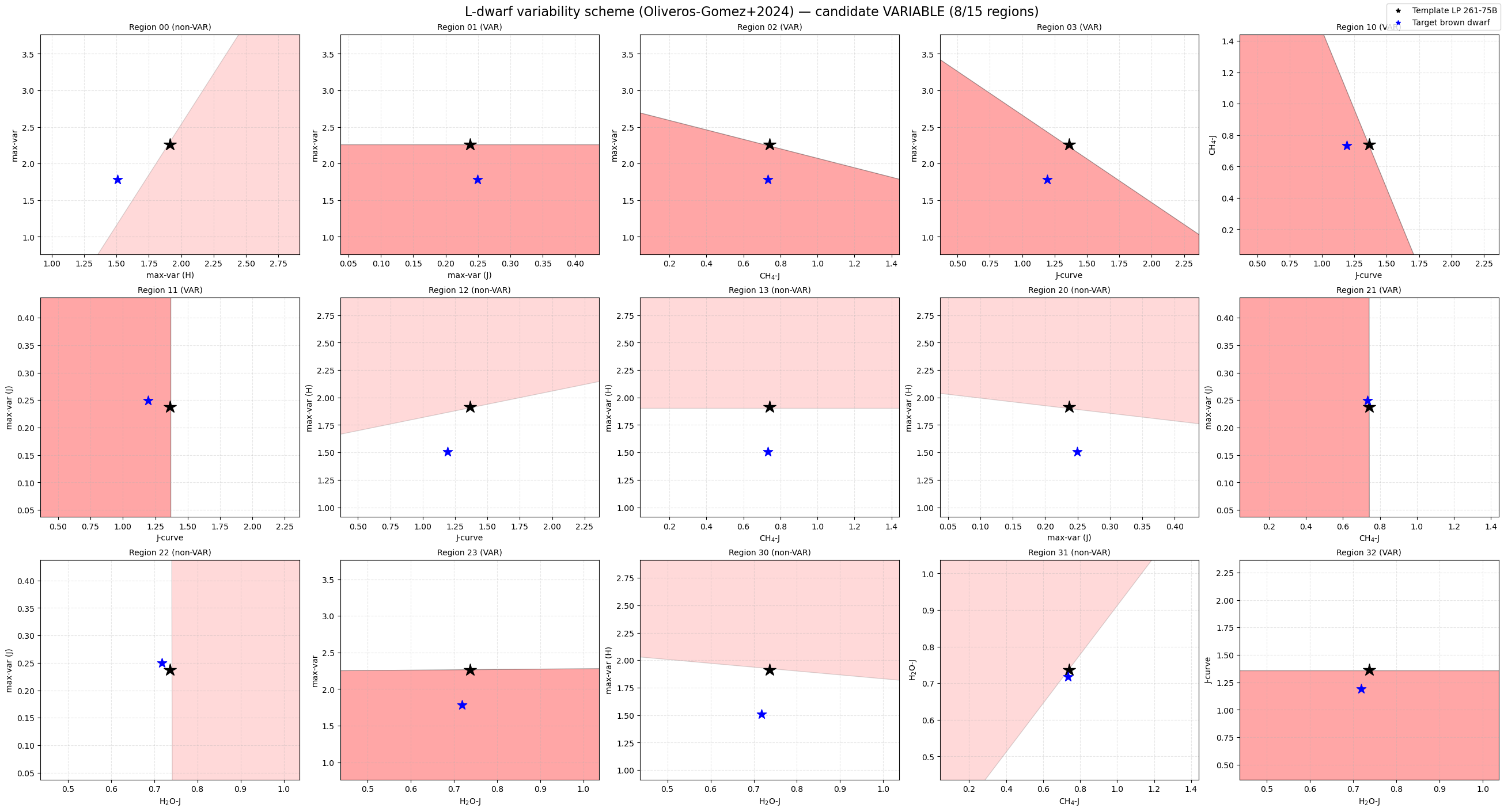
True
8 / 15
{'mostH': 1.5087388779766489, 'mostJ': 0.24971511702040977, 'less': 1.781314374877187, 'Jcurve': 1.192644800500469, 'H2OJ': 0.718355884207247, 'CH4J': 0.7325891829647628}
['01', '02', '03', '10', '11', '21', '23', '32']
Scheme: Oliveros-Gomez+2024
Spectral type: L
Triggered regions: 8/15 (threshold ≥ 8)
Classification: candidate VARIABLE

The most relevant attributes are:

• result.is_candidate_variable Final classification flag.

• result.n_regions_triggered Number of variability regions in which the target falls.

• result.n_regions_total Total number of regions considered for the selected spectral-type scheme.

• result.indices Dictionary containing the computed NIR spectral indices.

• result.regions_triggered List of region identifiers triggered by the target.

• result.summary() Human-readable summary of the classification.

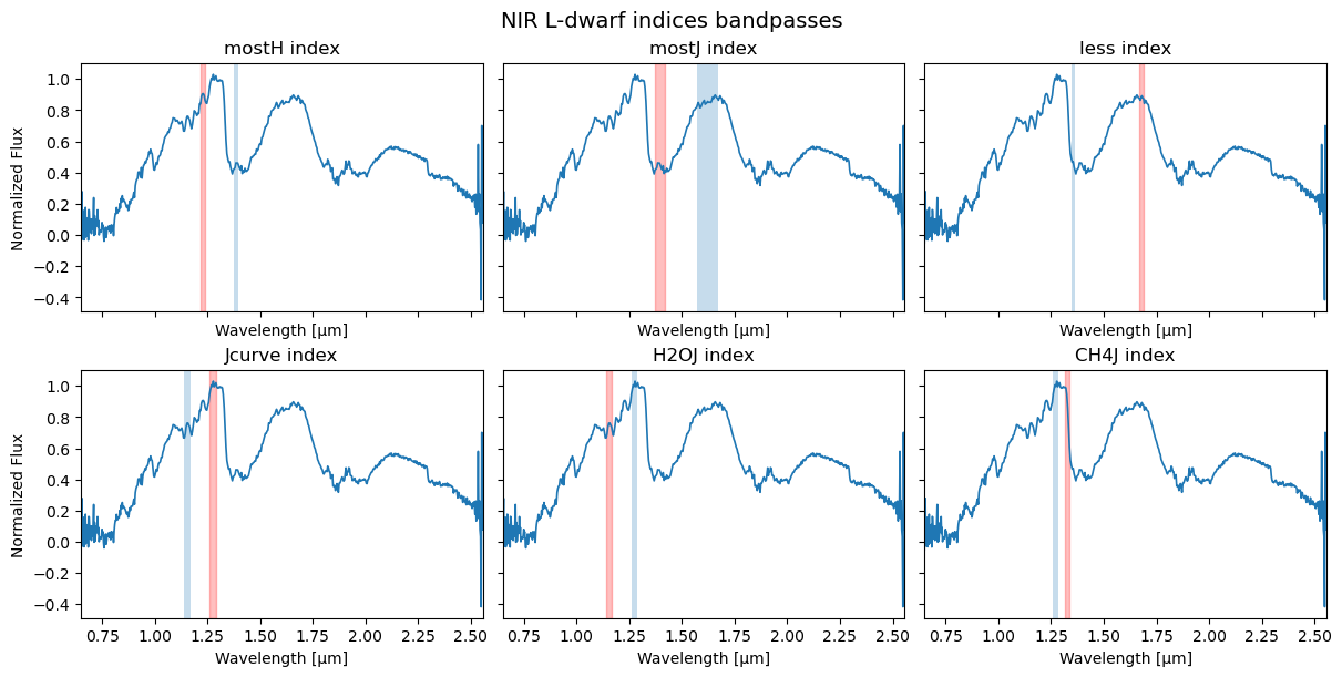
Plot the index bandpasses used in the classification

To visualize the spectral regions used to compute the variability indices, set plot_index_windows=True.

result = classify_variability(
    wave,
    flux,
    spectral_type="L",
    normalize=False,
    plot_index_windows=True,
)

This produces a multi-panel figure showing the input spectrum and the numerator/denominator wavelength windows used for each index in the selected L- or T-dwarf scheme.

If desired, the figure can be saved automatically:

Plot the index–index variability diagrams

To reproduce the variability classification diagrams, set plot_diagrams=True.

result = classify_variability(
    wave,
    flux,
    spectral_type="L",
    normalize=False,
    plot_diagrams=True,
)

These diagrams show:

• the polygonal variability regions,

• the template/reference object,

• and the position of the target object in index–index space.

You can also save the figure:

result = classify_variability(
    wave,
    flux,
    spectral_type="L",
    normalize=False,
    plot_diagrams=True,
    plot_save=True,
)

Generate both diagnostic plots at once

Both the index-window plot and the index–index diagrams can be generated in a single call:

result = classify_variability(
    wave,
    flux,
    spectral_type="L",
    normalize=False,
    plot_index_windows=True,
    plot_diagrams=True,
)

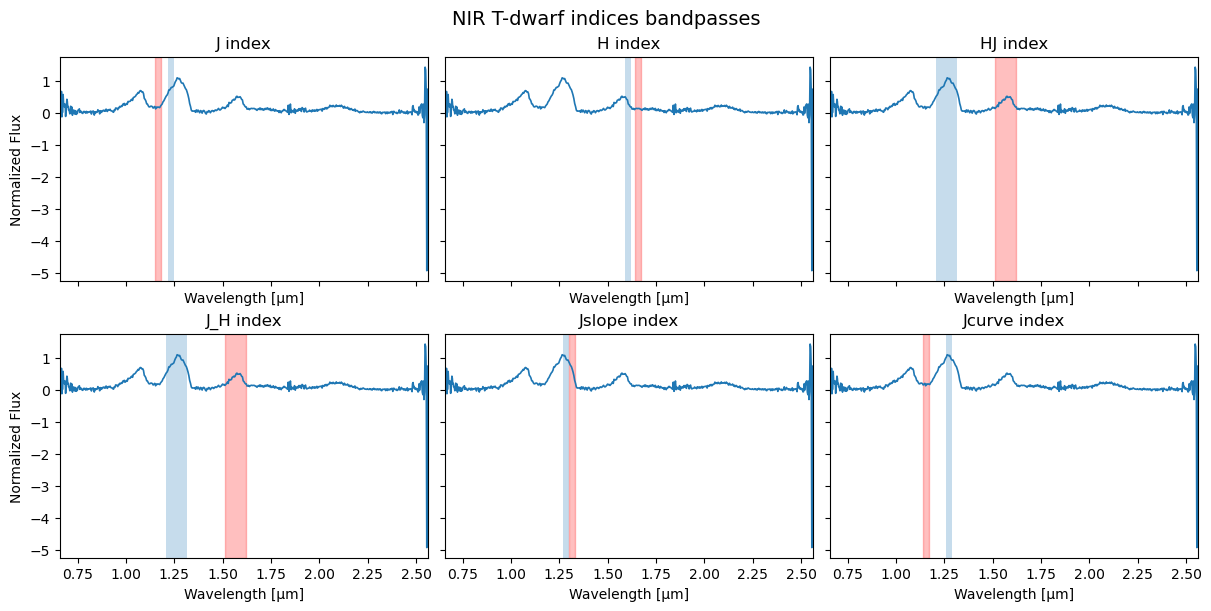
Example using the T-dwarf scheme

The same workflow applies to T dwarfs by changing the selected spectral type:

# read the T-dwarf spectrum
spec_name = '/Users/arrecifecosmico/seda/docs/notebooks/data/2228-nirspec-Tdwarf.txt'
spec = np.loadtxt(spec_name, comments='#').T

wave = spec[0]   # wavelength in microns
flux = spec[1]   # flux

result_T = classify_variability(
    wave,
    flux,
    spectral_type="T",
    normalize=False,
    plot_index_windows=True,
    plot_diagrams=True,
)

print(result_T.summary())

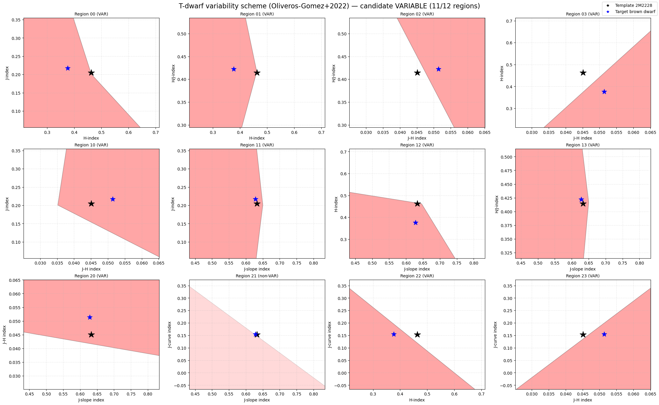
Scheme: Oliveros-Gomez+2022
Spectral type: T
Triggered regions: 11/12 (threshold ≥ 10)
Classification: candidate VARIABLE

Notes on normalization

The normalize parameter should be chosen consistently with the input spectrum and the intended use of the indices.

• If the spectrum is already normalized, use normalize=False.

• If the spectrum is not normalized and you want SEDA to apply a median normalization, use normalize=True.

This is especially important for difference-type indices, whose absolute scale depends on the adopted normalization.

Summary

seda.classify_variability provides a single high-level entry point to:

• compute the NIR variability indices,

• classify the target as candidate variable or non-variable,

• inspect the numerical results,

• and generate diagnostic plots.

This makes it straightforward to apply the variability scheme to individual L and T brown dwarf spectra.