Note

📥 Download this tutorial

Compute synthetic photometry for any SVO filters

Obtain synthetic photometry for any photometric filters in SVO and visualize the results.

import seda
import os
from astropy.io import fits, ascii
import matplotlib.pyplot as plt

    SEDA v0.5.6.dev3 package imported

Read the spectrum

As an example here, let’s read the near-infrared IRTF/SpeX spectrum for the T8 (~750 K) brown dwarf 2MASS J04151954-0935066 in Burgasser et al. (2004):

# path to the seda package
path_seda = os.path.dirname(os.path.dirname(seda.__file__))

# SpeX spectrum
SpeX_name = path_seda+'/docs/notebooks/data/0415-0935_IRTF_SpeX.dat'
SpeX = ascii.read(SpeX_name)
wl_SpeX = SpeX['wl(um)'] # um
flux_SpeX = SpeX['flux(erg/s/cm2/A)'] # erg/s/cm2/A
eflux_SpeX = SpeX['eflux(erg/s/cm2/A)'] # erg/s/cm2/A

Derive synthetic photometry

Obtain synthetic photometry for photometric filters with spectral coverage using SVO filter IDs.

# define filter IDs
filters = (['PAN-STARRS/PS1.y',
            'UKIRT/UKIDSS.Y', 'UKIRT/UKIDSS.J', 'UKIRT/UKIDSS.H', 'UKIRT/UKIDSS.K',
            '2MASS/2MASS.J', '2MASS/2MASS.H', '2MASS/2MASS.Ks']) # filters of interest

# obtain synthetic photometry
out = seda.synthetic_photometry.synthetic_photometry(wl=wl_SpeX,
                                                     flux=flux_SpeX,
                                                     eflux=eflux_SpeX,
                                                     flux_unit='erg/s/cm2/A',
                                                     filters=filters)

WARNING: UnitsWarning: The unit 'Angstrom' has been deprecated in the VOUnit standard. Suggested: 0.1nm. [astropy.units.format.utils]

   Caveat: No full spectral coverage for PAN-STARRS/PS1.y, so the synthetic photometry is a lower limit
      approx. 99.99% of the filter transmission is covered by the data

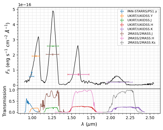
Plot results

Plot and save the input spectrum with the computed synthetic fluxes

Note that the PAN-STARRS/PS1.y flux is properly indicated as a lower limit.

fig, axs = seda.plots.plot_synthetic_photometry(out, save=True)

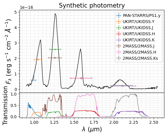
Plot and customize the plot generated above

fig, axs = seda.plots.plot_synthetic_photometry(out)

# improve legend
axs[0].legend(prop={'size': 10.0}, handlelength=1, handletextpad=0.5, labelspacing=0.5)

# set plot title
axs[0].set_title('Synthetic photometry', fontsize=15)

# increase font size of axes
axs[0].yaxis.label.set_size(15)
axs[1].yaxis.label.set_size(15)
axs[1].xaxis.label.set_size(15)

# export plot as PDF
plt.savefig(f'synthetic_photometry.pdf', bbox_inches='tight') # export plot as PDF
plt.show()