Nested sampling for spectrophotometric data
Forward modeling of an SED assembled from multiple spectra and photometry using the dynesty Bayesian framework and modern atmospheric models.
[1]:
import seda # import the seda package
import importlib
import numpy as np
import matplotlib.pyplot as plt
import os
import pickle
from matplotlib.ticker import MultipleLocator, FormatStrFormatter, AutoMinorLocator, StrMethodFormatter, NullFormatter
from astropy.io import fits, ascii
from dynesty import plotting as dyplot # to plot nested sampling results
SEDA v0.5.6.dev3 package imported
Read the data
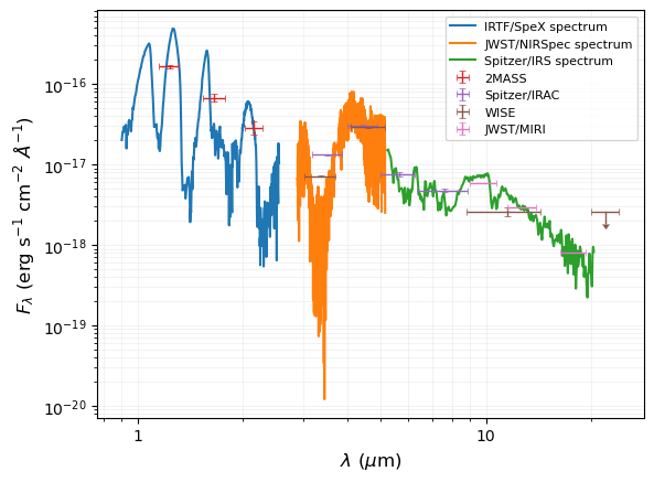
As an example here, let’s use:
Spectra: the near-infrared IRTF/SpeX, the mid-infrared JWST/NIRSpec, and the mid-infrared Spitzer/IRS spectra for the T8 (~750 K) brown dwarf 2MASS J04151954-0935066 in Burgasser et al. (2004), Alejandro Merchan et al. (2025), and Suárez & Metchev (2022), respectively.
Photometry: near- and mid-infrared magnitudes from different surveys (2MASS, Spitzer/IRAC, WISE, and JWST/MIRI) for the T8 (~750 K) brown dwarf 2MASS J04151954-0935066, as compiled in Alejandro Merchan et al. (2025):
Spectra
SpeX spectrum:
[2]:
# path to the seda package
path_seda = os.path.dirname(os.path.dirname(seda.__file__))

# SpeX spectrum
SpeX_name = path_seda+'/docs/notebooks/data/0415-0935_IRTF_SpeX.dat'
SpeX = ascii.read(SpeX_name)
wl_SpeX = SpeX['wl(um)'] # um
flux_SpeX = SpeX['flux(erg/s/cm2/A)'] # erg/s/cm2/A
eflux_SpeX = SpeX['eflux(erg/s/cm2/A)'] # erg/s/cm2/A
Read JWST NIRSpec spectrum
[3]:
NIRSpec_name = path_seda+'/docs/notebooks/data/0415-0935_NIRSpec_spectrum.dat'
NIRSpec = ascii.read(NIRSpec_name)
wl_NIRSpec = NIRSpec['wl(um)'] # um
flux_NIRSpec = NIRSpec['flux(Jy)'] # Jy
eflux_NIRSpec = NIRSpec['eflux(Jy)'] # Jy

# convert NIRSpec fluxes from Jy to erg/s/cm2/A
out_convert_flux = seda.synthetic_photometry.convert_flux(wl=wl_NIRSpec,
                                                          flux=flux_NIRSpec,
                                                          eflux=eflux_NIRSpec,
                                                          unit_in='Jy',
                                                          unit_out='erg/s/cm2/A')
flux_NIRSpec = out_convert_flux['flux_out'] # in erg/s/cm2/A
eflux_NIRSpec = out_convert_flux['eflux_out'] # in erg/s/cm2/A

# remove a few negative fluxes and edge points
mask = (flux_NIRSpec>0) & ((wl_NIRSpec<3.68) | (wl_NIRSpec>3.79))
wl_NIRSpec = wl_NIRSpec[mask]
flux_NIRSpec = flux_NIRSpec[mask]
eflux_NIRSpec = eflux_NIRSpec[mask]
Read IRS spectrum:
[4]:
IRS_name = path_seda+'/docs/notebooks/data/0415-0935_IRS_spectrum.dat'
IRS = ascii.read(IRS_name)
wl_IRS = IRS['wl(um)'] # in um
flux_IRS = IRS['flux(Jy)'] # in Jy
eflux_IRS = IRS['eflux(Jy)'] # in Jy

# convert IRS fluxes from Jy to erg/s/cm2/A
out_convert_flux = seda.synthetic_photometry.convert_flux(wl=wl_IRS,
                                                          flux=flux_IRS,
                                                          eflux=eflux_IRS,
                                                          unit_in='Jy',
                                                          unit_out='erg/s/cm2/A')
flux_IRS = out_convert_flux['flux_out'] # in erg/s/cm2/A
eflux_IRS = out_convert_flux['eflux_out'] # in erg/s/cm2/A
Photometry
[5]:
# path to the seda package
path_seda = os.path.dirname(os.path.dirname(seda.__file__))

# read table with photometry
phot_file = path_seda+'/docs/notebooks/data/0415-0935_photometry.dat'
photometry = ascii.read(phot_file)

# keep columns with magnitudes of interest
photometry.remove_column('WISE_designation') # remove only columns without photometry

# convert table with photometry to a dictionary with three keys: filters, photometry, and uncertainties
# save output dictionary as a fancy ascii table in the seda directory "data"
# the output table can be open using "seda.read_prettytable"
table_name = path_seda+'/docs/notebooks/data/0415-0935_photometry_prettytable.dat'
out = seda.utils.convert_photometric_table(photometry, save_table=True,
                                           table_name=table_name)
phot = out['phot']
ephot = out['ephot']
filters = out['filters']
Convert magnitudes into fluxes:
[7]:
# mag to flux
out_mag_to_flux = seda.synthetic_photometry.mag_to_flux(mag=phot,
                                                        emag=ephot,
                                                        filters=filters,
                                                        flux_unit='erg/s/cm2/A')
flux = out_mag_to_flux['flux'] # in erg/s/cm2/A
eflux = out_mag_to_flux['eflux'] # in erg/s/cm2/A
wl_eff = out_mag_to_flux['lambda_eff_SVO(um)'] # effective wavelength in um
width_eff = out_mag_to_flux['width_eff_SVO(um)'] # effective width in um
filters = out_mag_to_flux['filters']
Plot SED
Plot the data to verify everything looks okay:
[8]:
fig, ax = plt.subplots()

# plot spectra
plt.plot(wl_SpeX, flux_SpeX, label='IRTF/SpeX spectrum')
plt.plot(wl_NIRSpec, flux_NIRSpec, label='JWST/NIRSpec spectrum')
plt.plot(wl_IRS, flux_IRS, label='Spitzer/IRS spectrum')

# plot photometry
# select 2MASS magnitudes
mask_2MASS = ['2MASS' in filt for filt in filters]
ax.errorbar(wl_eff[mask_2MASS], flux[mask_2MASS], xerr=width_eff[mask_2MASS]/2,
            yerr=eflux[mask_2MASS], fmt='.', markersize=1., capsize=2,
            elinewidth=1.0, markeredgewidth=0.5, label='2MASS')

# select IRAC magnitudes
mask_IRAC = ['IRAC' in filt for filt in filters]
ax.errorbar(wl_eff[mask_IRAC], flux[mask_IRAC], xerr=width_eff[mask_IRAC]/2,
            yerr=eflux[mask_IRAC], fmt='.', markersize=1., capsize=2,
            elinewidth=1.0, markeredgewidth=0.5, label='Spitzer/IRAC')

# select WISE magnitudes
mask_WISE = ['WISE' in filt for filt in filters]
# handle upper limits
uplims = (ephot==0) * 1 # upper limits (null errors) indicated by 1
eflux[eflux==0] = 0.3*flux[eflux==0] # size of the arrow indicating upper limits
# plot WISE with upper limits
ax.errorbar(wl_eff[mask_WISE], flux[mask_WISE], xerr=width_eff[mask_WISE]/2,
            yerr=eflux[mask_WISE], fmt='.', markersize=1., capsize=2,
            elinewidth=1.0, markeredgewidth=0.5, label='WISE',
            uplims=uplims[mask_WISE])

# select MIRI magnitudes
mask_JWST = ['JWST' in filt for filt in filters]
ax.errorbar(wl_eff[mask_JWST], flux[mask_JWST], xerr=width_eff[mask_JWST]/2,
            yerr=eflux[mask_JWST], fmt='.', markersize=1., capsize=2,
            elinewidth=1.0, markeredgewidth=0.5, label='JWST/MIRI')

ax.xaxis.set_minor_locator(AutoMinorLocator())
ax.yaxis.set_minor_locator(AutoMinorLocator())
plt.xscale('log')
plt.yscale('log')
ax.xaxis.set_major_formatter(StrMethodFormatter('{x:.0f}'))

ax.grid(True, which='both', color='gainsboro', linewidth=0.5, alpha=0.5)
ax.legend(fontsize=8)

plt.xlabel(r'$\lambda\ (\mu$m)', size=12)
plt.ylabel(r'$F_\lambda\ ($erg s$^{-1}$ cm$^{-2}$ $\AA^{-1}$)', size=12)

plt.show()
Load input data
Look at the input parameters here.
For any SEDA function, we can also see the function description directly on the notebook with the command help(), e.g.:
help(seda.input_parameters.InputData)
[9]:
# spectra
#--------
# wavelenghts
wl_spectra = [wl_SpeX, wl_NIRSpec, wl_IRS] # in um
# fluxes
flux_spectra = [flux_SpeX, flux_NIRSpec, flux_IRS] # in erg/s/cm2/A
# flux uncertainties
eflux_spectra = [eflux_SpeX, eflux_NIRSpec, eflux_IRS] # in erg/s/cm2/A
# specify flux units
flux_unit = 'erg/s/cm2/A'

# resolution of each input spectrum (used to convolve the model spectra)
res = [100, 2700, 100] # SpeX, NIRSpec, IRS

# photometry
#-----------
# input photometry
phot = phot
ephot = ephot
filters = filters
phot_unit = 'mag'

# distance to the target (optional and used to derive a radius)
distance = 5.71 # pc (parallax=175.2+-1.7; Dupuy-Liu2012)
edistance = 0.06 # pc

# load all the input data parameters
my_data = seda.input_parameters.InputData(wl_spectra=wl_spectra,
                                          flux_spectra=flux_spectra,
                                          eflux_spectra=eflux_spectra,
                                          flux_unit=flux_unit,
                                          res=res,
                                          phot=phot,
                                          ephot=ephot,
                                          filters=filters,
                                          phot_unit=phot_unit,
                                          fit_photometry=True,
                                          distance=distance,
                                          edistance=edistance)
Null photometric errors for ['WISE/WISE.W4'] magnitudes, so they will be discarded.

   Input data loaded successfully:
      3 spectra
      13 magnitudes
Download (if not yet) the atmospheric models you want to use.
Use the commands below to see the available atmospheric models, the links to download them, and other relevant information from models. You can read more about the model here.
Also consider this tutorial to explore the free parameters in the models and their coverage.
[10]:
# available atmospheric models
seda.models.Models().available_models
[10]:
['BT-Settl',
 'ATMO2020',
 'Sonora_Elf_Owl',
 'SM08',
 'Sonora_Bobcat',
 'Sonora_Diamondback',
 'Sonora_Cholla',
 'LB23']
[11]:
# some parameters of interest from a selected model
model = 'Sonora_Elf_Owl'
print(seda.models.Models(model).ref) # reference
print(seda.models.Models(model).ADS) # link to paper
print(seda.models.Models(model).download) # link to download the models
seda.models.Models(model).params_unique # coverage of free parameters in the grid
Mukherjee et al. (2024)
https://ui.adsabs.harvard.edu/abs/2024ApJ...963...73M/abstract
['https://zenodo.org/records/10385987', 'https://zenodo.org/records/10385821', 'https://zenodo.org/records/10381250']
[11]:
{'Teff': array([ 275.,  300.,  325.,  350.,  375.,  400.,  425.,  450.,  475.,
         500.,  525.,  550.,  575.,  600.,  650.,  700.,  750.,  800.,
         850.,  900.,  950., 1000., 1100., 1200., 1300., 1400., 1500.,
        1600., 1700., 1800., 1900., 2000., 2100., 2200., 2300., 2400.]),
 'logg': array([3.  , 3.25, 3.5 , 3.75, 4.  , 4.25, 4.5 , 4.75, 5.  , 5.25, 5.5 ]),
 'logKzz': array([2., 4., 7., 8., 9.]),
 'Z': array([-1. , -0.5,  0. ,  0.5,  0.7,  1. ]),
 'CtoO': array([0.5, 1. , 1.5, 2. , 2.5])}
Load model grid options
Look at the input parameters here.
[12]:
# select the atmospheric models of interest
model = 'Sonora_Elf_Owl'

# path to the directory or directories containing the model spectra
# (update it to your own path)
my_path = '/home/gsuarez/TRABAJO/MODELS/atmosphere_models/Sonora_Elf_Owl/spectra/'
model_dir = [my_path+'output_700.0_800.0/',
             my_path+'output_850.0_950.0/',
            ]

# set parameter ranges to select a grid subset and to be used as uniform priors
# when a free parameter range is not specified, the whole grid range will be considered
params_ranges = {
    'Teff': [700, 900], # Teff range
    'logg': [4.0, 5.0], # logg range
}

# load model options
my_model = seda.input_parameters.ModelOptions(model=model, model_dir=model_dir,
                                              params_ranges=params_ranges)
Model options loaded successfully
Tip: If you plan to model several spectra from the same instrument (same resolution), you can save the convolved model spectra to reuse them and do subsequent fits much faster. For this, set the parameter path_save_spectra_conv in seda.ModelOptions above to a folder path where you want to store the convolved spectra. Once the spectra are stored, the next time you run the code just replace model_dir by the path you used in path_save_spectra_conv and set
skip_convolution=True to avoid the model convolution. This was implemented thanks to this issue.
Load Bayes fit options
Look at the input parameters here.
Consider the default full wavelength range of each input spectrum for the fits. Otherwise, we can use the parameter fit_wl_range to set different fit ranges.
[13]:
# choose a filename (optional) to save the sampling results as a pickle file
# it is convenient to set a non-default name when running
# the code several times in the same folder to avoid overwriting results
bayes_pickle_file = f'{model}_bayesian_sampling_spectrophotometry.pickle'

# radius range for the sampling
R_range = np.array((0.6, 1.0)) # Rjup

my_bayes = seda.input_parameters.BayesOptions(my_data=my_data,
                                              my_model=my_model,
                                              R_range=R_range,
                                              bayes_pickle_file=bayes_pickle_file)
For input spectrum 1 of 3

      3000 model spectra selected with:
         Teff range = [700, 900]
         logg range = [4.0, 5.0]
      elapsed time: 6.0 min

For input spectrum 2 of 3

      3000 model spectra selected with:
         Teff range = [700, 900]
         logg range = [4.0, 5.0]
      elapsed time: 2.1 min

For input spectrum 3 of 3

      3000 model spectra selected with:
         Teff range = [700, 900]
         logg range = [4.0, 5.0]
      elapsed time: 5.4 min

      11/13 selected input magnitudes within "fit_phot_range" or the model wavelength range

         Filters ['WISE/WISE.W3' 'JWST/MIRI.F1800W'] are outside the "fit_phot_range" or the model wavelength range, so they will be ignored in the fits.

      3000 model spectra selected with:
         Teff range = [700, 900]
         logg range = [4.0, 5.0]
      elapsed time: 2.6 hr

   Bayes fit options loaded successfully
Run nested sampling
[14]:
out_bayes = seda.bayes_fit.bayes(my_bayes)
   Estimate Bayesian posteriors

      Uniform priors:
         Teff range = [700. 900.]
         logg range = [4. 5.]
         logKzz range = [2. 9.]
         Z range = [-1.  1.]
         CtoO range = [0.5 2.5]
         R range = [0.6 1. ]

   Starting dynesty...
20258it [39:46, 8.49it/s, batch: 5 | bound: 15 | nc: 1 | ncall: 99033 | eff(%): 20.157 | loglstar: 156811.721 < 156818.420 < 156816.911 | logz: 156798.802 +/- 0.131 | stop: 0.847]
      Bayesian sampling results saved successfully

   Bayesian sampling ran successfully
      elapsed time: 39.8 min
Plot results
The out_bayes output above from seda.bayes_fit.bayes is the input file to make plots.
If out_bayes is not in memory (if we reloaded the notebook or restarted the kernel), we need to open the pickle file first as below.
[8]:
# open pickle file
bayes_pickle_file = 'Sonora_Elf_Owl_bayesian_sampling_spectrophotometry.pickle'
with open(bayes_pickle_file, 'rb') as file:
    # deserialize and retrieve the variable from the file
    out_bayes = pickle.load(file)

print('Posteriors loaded successfully')
Posteriors loaded successfully
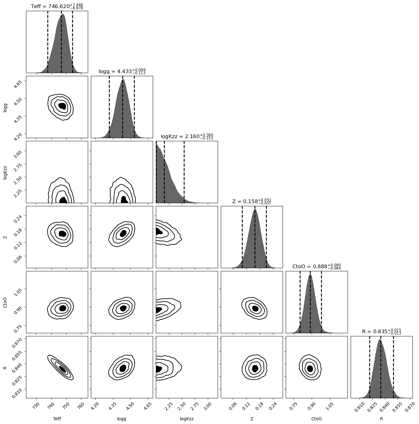
[16]:
# plot the 2-D marginalized posteriors.
labels = list(out_bayes['my_bayes'].params_priors.keys())
fig, axes = dyplot.cornerplot(out_bayes['out_dynesty'], show_titles=True,
                              verbose='true', title_fmt='.3f',
                              title_kwargs={'y': 1.0}, labels=labels)
Quantiles:
Teff [(0.025, 737.6425713697995), (0.5, 746.6203786116977), (0.975, 754.088204821028)]
Quantiles:
logg [(0.025, 4.3201175321727305), (0.5, 4.432617810342954), (0.975, 4.532035545888423)]
Quantiles:
logKzz [(0.025, 2.007633391389391), (0.5, 2.1601682147021455), (0.975, 2.540566178745848)]
Quantiles:
Z [(0.025, 0.10113725668174171), (0.5, 0.15818796767994772), (0.975, 0.20926829818877749)]
Quantiles:
CtoO [(0.025, 0.8042059154841594), (0.5, 0.8884503528771852), (0.975, 0.9780460151758429)]
Quantiles:
R [(0.025, 0.8216888227058947), (0.5, 0.8349010336288848), (0.975, 0.850191651122284)]
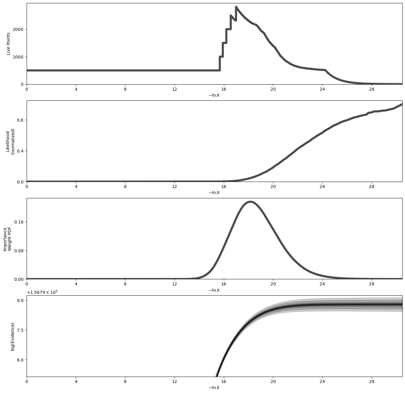
Plot a summary of the run
[17]:
fig, axes = dyplot.runplot(out_bayes['out_dynesty'], color='black',
                           mark_final_live=False, logplot=True)
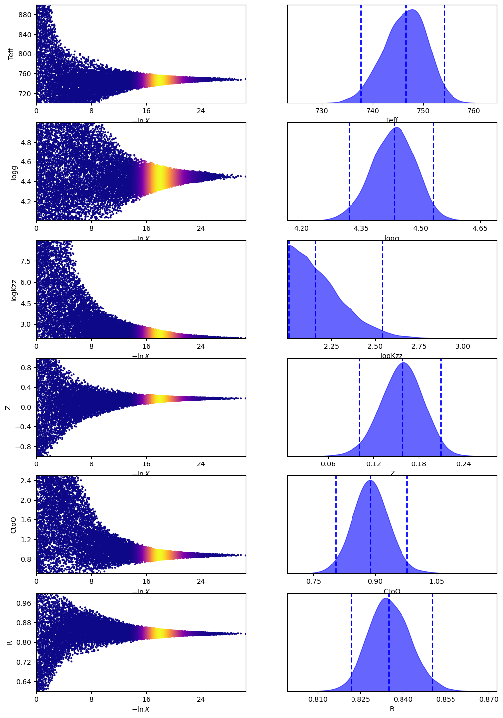
Plot traces and 1-D marginalized posteriors
[18]:
fig, axes = dyplot.traceplot(out_bayes['out_dynesty'], labels=labels)
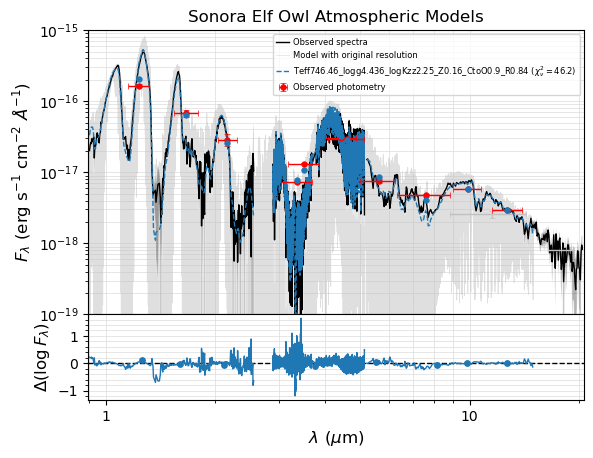
Plot the model spectrum using the median posterior parameters
SED with the best model fit from the Bayesian sampling.
The pickle file generated by seda.bayes_fit.bayes and stored with the name my_bayes.bayes_pickle_file is the input file to make plots. We can provide the name by either using my_bayes.bayes_pickle_file (if my_bayes is in memory) or just typing it.
The best model fit will be generated by interpolating into a model grid subset around the median posteriors.
[9]:
# using default logarithmic scale for fluxes
fig, ax = seda.plots.plot_bayes_fit(bayes_pickle_file, xlog=True,
                                    yrange=[1e-19, 1e-15],
                                    ori_res=True)
For input spectrum 1 of 3

      32 model spectra selected with:
         Teff range = [700. 750.]
         logg range = [4.25 4.5 ]
         logKzz range = [2. 4.]
         Z range = [0.  0.5]
         CtoO range = [0.5 1. ]
      elapsed time: 4.0 s

For input spectrum 2 of 3

      32 model spectra selected with:
         Teff range = [700. 750.]
         logg range = [4.25 4.5 ]
         logKzz range = [2. 4.]
         Z range = [0.  0.5]
         CtoO range = [0.5 1. ]
      elapsed time: 1.0 s

For input spectrum 3 of 3

      32 model spectra selected with:
         Teff range = [700. 750.]
         logg range = [4.25 4.5 ]
         logKzz range = [2. 4.]
         Z range = [0.  0.5]
         CtoO range = [0.5 1. ]
      elapsed time: 3.0 s

      32 model spectra selected with:
         Teff range = [700. 750.]
         logg range = [4.25 4.5 ]
         logKzz range = [2. 4.]
         Z range = [0.  0.5]
         CtoO range = [0.5 1. ]
      elapsed time: 1.8 min

      7206 model spectra

      32 model spectra selected with:
         Teff range = [700. 750.]
         logg range = [4.25 4.5 ]
         logKzz range = [2. 4.]
         Z range = [0.  0.5]
         CtoO range = [0.5 1. ]
elapsed time: 0.0 s
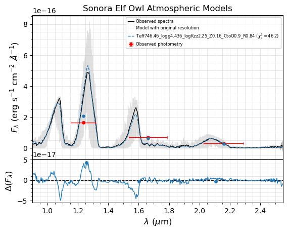
Zoom in on the SpeX spectrum:
[10]:
# plot fluxes in linear scale
fig, ax = seda.plots.plot_bayes_fit(bayes_pickle_file, ylog=False,
                                    xrange=[wl_SpeX.min(), wl_SpeX.max()],
                                    ori_res=True)
For input spectrum 1 of 3

      32 model spectra selected with:
         Teff range = [700. 750.]
         logg range = [4.25 4.5 ]
         logKzz range = [2. 4.]
         Z range = [0.  0.5]
         CtoO range = [0.5 1. ]
      elapsed time: 4.0 s

For input spectrum 2 of 3

      32 model spectra selected with:
         Teff range = [700. 750.]
         logg range = [4.25 4.5 ]
         logKzz range = [2. 4.]
         Z range = [0.  0.5]
         CtoO range = [0.5 1. ]
      elapsed time: 1.0 s

For input spectrum 3 of 3

      32 model spectra selected with:
         Teff range = [700. 750.]
         logg range = [4.25 4.5 ]
         logKzz range = [2. 4.]
         Z range = [0.  0.5]
         CtoO range = [0.5 1. ]
      elapsed time: 6.0 s

      32 model spectra selected with:
         Teff range = [700. 750.]
         logg range = [4.25 4.5 ]
         logKzz range = [2. 4.]
         Z range = [0.  0.5]
         CtoO range = [0.5 1. ]
WARNING: UnitsWarning: The unit 'Angstrom' has been deprecated in the VOUnit standard. Suggested: 0.1nm. [astropy.units.format.utils]
      elapsed time: 3.6 min

      7206 model spectra

      32 model spectra selected with:
         Teff range = [700. 750.]
         logg range = [4.25 4.5 ]
         logKzz range = [2. 4.]
         Z range = [0.  0.5]
         CtoO range = [0.5 1. ]
elapsed time: 1.0 s
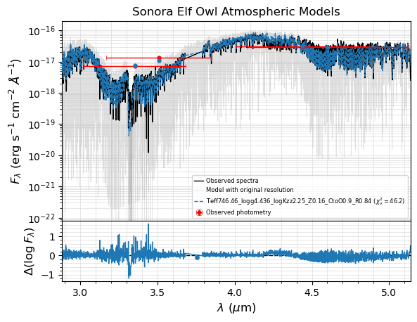
Zoom in on the NIRSpec spectrum:
[11]:
# plot fluxes in log scale
fig, ax = seda.plots.plot_bayes_fit(bayes_pickle_file,
                                    xrange=[wl_NIRSpec.min(), wl_NIRSpec.max()],
                                    ori_res=True)
For input spectrum 1 of 3

      32 model spectra selected with:
         Teff range = [700. 750.]
         logg range = [4.25 4.5 ]
         logKzz range = [2. 4.]
         Z range = [0.  0.5]
         CtoO range = [0.5 1. ]
      elapsed time: 7.0 s

For input spectrum 2 of 3

      32 model spectra selected with:
         Teff range = [700. 750.]
         logg range = [4.25 4.5 ]
         logKzz range = [2. 4.]
         Z range = [0.  0.5]
         CtoO range = [0.5 1. ]
      elapsed time: 3.0 s

For input spectrum 3 of 3

      32 model spectra selected with:
         Teff range = [700. 750.]
         logg range = [4.25 4.5 ]
         logKzz range = [2. 4.]
         Z range = [0.  0.5]
         CtoO range = [0.5 1. ]
      elapsed time: 6.0 s

      32 model spectra selected with:
         Teff range = [700. 750.]
         logg range = [4.25 4.5 ]
         logKzz range = [2. 4.]
         Z range = [0.  0.5]
         CtoO range = [0.5 1. ]
WARNING: UnitsWarning: The unit 'Angstrom' has been deprecated in the VOUnit standard. Suggested: 0.1nm. [astropy.units.format.utils]
      elapsed time: 3.4 min

      7206 model spectra

      32 model spectra selected with:
         Teff range = [700. 750.]
         logg range = [4.25 4.5 ]
         logKzz range = [2. 4.]
         Z range = [0.  0.5]
         CtoO range = [0.5 1. ]
elapsed time: 1.0 s
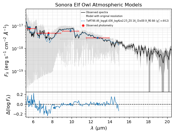
Zoom in on the IRS spectrum:
[12]:
# plot fluxes in log scale
fig, ax = seda.plots.plot_bayes_fit(bayes_pickle_file,
                                    xrange=[wl_IRS.min(), wl_IRS.max()],
                                    ori_res=True)
For input spectrum 1 of 3

      32 model spectra selected with:
         Teff range = [700. 750.]
         logg range = [4.25 4.5 ]
         logKzz range = [2. 4.]
         Z range = [0.  0.5]
         CtoO range = [0.5 1. ]
      elapsed time: 5.0 s

For input spectrum 2 of 3

      32 model spectra selected with:
         Teff range = [700. 750.]
         logg range = [4.25 4.5 ]
         logKzz range = [2. 4.]
         Z range = [0.  0.5]
         CtoO range = [0.5 1. ]
      elapsed time: 1.0 s

For input spectrum 3 of 3

      32 model spectra selected with:
         Teff range = [700. 750.]
         logg range = [4.25 4.5 ]
         logKzz range = [2. 4.]
         Z range = [0.  0.5]
         CtoO range = [0.5 1. ]
      elapsed time: 4.0 s

      32 model spectra selected with:
         Teff range = [700. 750.]
         logg range = [4.25 4.5 ]
         logKzz range = [2. 4.]
         Z range = [0.  0.5]
         CtoO range = [0.5 1. ]
WARNING: UnitsWarning: The unit 'Angstrom' has been deprecated in the VOUnit standard. Suggested: 0.1nm. [astropy.units.format.utils]
      elapsed time: 1.9 min

      7206 model spectra

      32 model spectra selected with:
         Teff range = [700. 750.]
         logg range = [4.25 4.5 ]
         logKzz range = [2. 4.]
         Z range = [0.  0.5]
         CtoO range = [0.5 1. ]
elapsed time: 0.0 s
[ ]: