Nested sampling for multiple spectra of the same object
Forward modeling of multiple spectra for the same object using modern atmospheric models and the dynesty Bayesian framework.
[1]:
import seda # import the seda package
import importlib
import numpy as np
import matplotlib.pyplot as plt
import pickle
import os
from matplotlib.ticker import MultipleLocator, FormatStrFormatter, AutoMinorLocator, StrMethodFormatter, NullFormatter
from astropy.io import fits, ascii
from dynesty import plotting as dyplot # to plot nested sampling results
SEDA v0.5.6.dev3 package imported
Read the spectra
As an example here, let’s read the near-infrared IRTF/SpeX, the mid-infrared JWST/NIRSpec, and the mid-infrared Spitzer/IRS spectra for the T8 (~750 K) brown dwarf 2MASS J04151954-0935066 in Burgasser et al. (2004), Alejandro Merchan et al. (2025) and Suárez & Metchev (2022), respectively.
Read SpeX spectrum:
[2]:
# path to the seda package
path_seda = os.path.dirname(os.path.dirname(seda.__file__))

SpeX_name = path_seda+'/docs/notebooks/data/0415-0935_IRTF_SpeX.dat'
SpeX = ascii.read(SpeX_name)
wl_SpeX = SpeX['wl(um)'] # um
flux_SpeX = SpeX['flux(erg/s/cm2/A)'] # erg/s/cm2/A
eflux_SpeX = SpeX['eflux(erg/s/cm2/A)'] # erg/s/cm2/A
Read JWST NIRSpec spectrum
[3]:
NIRSpec_name = path_seda+'/docs/notebooks/data/0415-0935_NIRSpec_spectrum.dat'
NIRSpec = ascii.read(NIRSpec_name)
wl_NIRSpec = NIRSpec['wl(um)'] # um
flux_NIRSpec = NIRSpec['flux(Jy)'] # Jy
eflux_NIRSpec = NIRSpec['eflux(Jy)'] # Jy

# convert NIRSpec fluxes from Jy to erg/s/cm2/A
out_convert_flux = seda.synthetic_photometry.convert_flux(wl=wl_NIRSpec,
                                                          flux=flux_NIRSpec,
                                                          eflux=eflux_NIRSpec,
                                                          unit_in='Jy',
                                                          unit_out='erg/s/cm2/A')
flux_NIRSpec = out_convert_flux['flux_out'] # in erg/s/cm2/A
eflux_NIRSpec = out_convert_flux['eflux_out'] # in erg/s/cm2/A

# remove a few negative fluxes and edge points
mask = (flux_NIRSpec>0) & ((wl_NIRSpec<3.68) | (wl_NIRSpec>3.79))
wl_NIRSpec = wl_NIRSpec[mask]
flux_NIRSpec = flux_NIRSpec[mask]
eflux_NIRSpec = eflux_NIRSpec[mask]
Read IRS spectrum:
[4]:
IRS_name = path_seda+'/docs/notebooks/data/0415-0935_IRS_spectrum.dat'
IRS = ascii.read(IRS_name)
wl_IRS = IRS['wl(um)'] # in um
flux_IRS = IRS['flux(Jy)'] # in Jy
eflux_IRS = IRS['eflux(Jy)'] # in Jy

# convert IRS fluxes from Jy to erg/s/cm2/A
out_convert_flux = seda.synthetic_photometry.convert_flux(wl=wl_IRS, flux=flux_IRS,
                                                          eflux=eflux_IRS,
                                                          unit_in='Jy',
                                                          unit_out='erg/s/cm2/A')
flux_IRS = out_convert_flux['flux_out'] # in erg/s/cm2/A
eflux_IRS = out_convert_flux['eflux_out'] # in erg/s/cm2/A
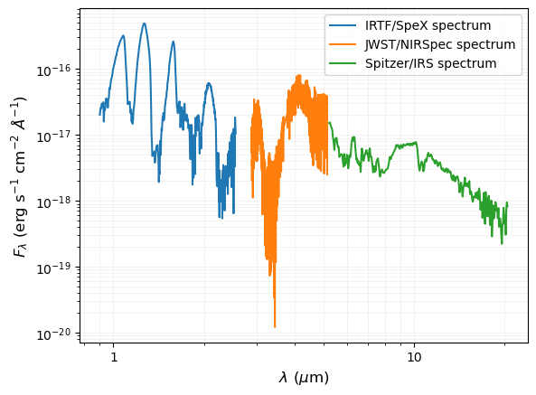
Plot SED to check everything looks okay:
[5]:
fig, ax = plt.subplots()

plt.plot(wl_SpeX, flux_SpeX, label='IRTF/SpeX spectrum')
plt.plot(wl_NIRSpec, flux_NIRSpec, label='JWST/NIRSpec spectrum')
plt.plot(wl_IRS, flux_IRS, label='Spitzer/IRS spectrum')

ax.xaxis.set_minor_locator(AutoMinorLocator())
ax.yaxis.set_minor_locator(AutoMinorLocator())
plt.xscale('log')
plt.yscale('log')
ax.xaxis.set_major_formatter(StrMethodFormatter('{x:.0f}'))

ax.grid(True, which='both', color='gainsboro', linewidth=0.5, alpha=0.5)
ax.legend()

plt.xlabel(r'$\lambda\ (\mu$m)', size=12)
plt.ylabel(r'$F_\lambda\ ($erg s$^{-1}$ cm$^{-2}$ $\AA^{-1}$)', size=12)

plt.show()
Load input data
Look at the input parameters here.
For any SEDA function, we can also see the function description directly on the notebook with the command help(), e.g.:
help(seda.input_parameters.InputData)
Define lists with the input spectra:
[7]:
# wavelenghts
wl_spectra = [wl_SpeX, wl_NIRSpec, wl_IRS] # in um
# fluxes
flux_spectra = [flux_SpeX, flux_NIRSpec, flux_IRS] # in erg/s/cm2/A
# flux uncertainties
eflux_spectra = [eflux_SpeX, eflux_NIRSpec, eflux_IRS] # in erg/s/cm2/A
# specify flux units
flux_unit = 'erg/s/cm2/A'

# resolution of each input spectrum (used to convolve the model spectra)
res = [100, 2700, 100] # SpeX, NIRSpec, IRS

# distance to the target (optional and used to derive a radius)
distance = 5.71 # pc (parallax=175.2+-1.7; Dupuy-Liu2012)
edistance = 0.06 # pc

# load all the input data parameters
my_data = seda.input_parameters.InputData(wl_spectra=wl_spectra,
                                          flux_spectra=flux_spectra,
                                          eflux_spectra=eflux_spectra,
                                          flux_unit=flux_unit,
                                          res=res, distance=distance,
                                          edistance=edistance)
   Input data loaded successfully:
      3 spectra
Download (if not yet) the atmospheric models you want to use.
Use the commands below to see the available atmospheric models, the links to download them, and other relevant information from models. You can read more about the model here.
Also consider this tutorial to explore the free parameters in the models and their coverage.
[8]:
# available atmospheric models
seda.models.Models().available_models
[8]:
['BT-Settl',
 'ATMO2020',
 'Sonora_Elf_Owl',
 'SM08',
 'Sonora_Bobcat',
 'Sonora_Diamondback',
 'Sonora_Cholla',
 'LB23']
[9]:
# some parameters of interest from a selected model
model = 'Sonora_Elf_Owl'
print(seda.models.Models(model).ref) # reference
print(seda.models.Models(model).ADS) # link to paper
print(seda.models.Models(model).download) # link to download the models
seda.models.Models(model).params_unique # coverage of free parameters in the grid
Mukherjee et al. (2024)
https://ui.adsabs.harvard.edu/abs/2024ApJ...963...73M/abstract
['https://zenodo.org/records/10385987', 'https://zenodo.org/records/10385821', 'https://zenodo.org/records/10381250']
[9]:
{'Teff': array([ 275.,  300.,  325.,  350.,  375.,  400.,  425.,  450.,  475.,
         500.,  525.,  550.,  575.,  600.,  650.,  700.,  750.,  800.,
         850.,  900.,  950., 1000., 1100., 1200., 1300., 1400., 1500.,
        1600., 1700., 1800., 1900., 2000., 2100., 2200., 2300., 2400.]),
 'logg': array([3.  , 3.25, 3.5 , 3.75, 4.  , 4.25, 4.5 , 4.75, 5.  , 5.25, 5.5 ]),
 'logKzz': array([2., 4., 7., 8., 9.]),
 'Z': array([-1. , -0.5,  0. ,  0.5,  0.7,  1. ]),
 'CtoO': array([0.5, 1. , 1.5, 2. , 2.5])}
Load model grid options
Look at the input parameters here.
[10]:
# select the atmospheric models of interest
model = 'Sonora_Elf_Owl'

# path to the directory or directories containing the model spectra
# (update it to your own path)
my_path = '/home/gsuarez/TRABAJO/MODELS/atmosphere_models/Sonora_Elf_Owl/spectra/'
model_dir = [my_path+'output_700.0_800.0/',
             my_path+'output_850.0_950.0/',
            ]

# set parameter ranges to select a grid subset and to be used as uniform priors
# when a free parameter range is not specified, the whole grid range will be considered
params_ranges = {
    'Teff': [700, 900], # Teff range
    'logg': [4.0, 5.0] # logg range
}

# load model options
my_model = seda.input_parameters.ModelOptions(model=model, model_dir=model_dir,
                                              params_ranges=params_ranges)
Model options loaded successfully
Tip: If you plan to model several spectra from the same instrument (same resolution), you can save the convolved model spectra to reuse them and do subsequent fits much faster. For this, set the parameter path_save_spectra_conv in seda.ModelOptions above to a folder path where you want to store the convolved spectra. Once the spectra are stored, the next time you run the code just replace model_dir by the path you used in path_save_spectra_conv and set
skip_convolution=True to avoid the model convolution. This was implemented thanks to issue.
Load Bayes fit options
Look at the input parameters here.
Consider the default full wavelength range of each input spectrum for the fits. Otherwise, we can use the parameter fit_wl_range to set different fit ranges.
[11]:
# choose a filename (optional) to save the sampling results as a pickle file
# it is convenient to set a non-default name when running
# the code several times in the same folder to avoid overwriting results
bayes_pickle_file = f'{model}_bayesian_sampling_multiple_spectra.pickle'

# radius range for the sampling
R_range = np.array((0.6, 1.0)) # Rjup

my_bayes = seda.input_parameters.BayesOptions(my_data=my_data, my_model=my_model,
                                              R_range=R_range,
                                              bayes_pickle_file=bayes_pickle_file)
For input spectrum 1 of 3

      3000 model spectra selected with:
         Teff range = [700, 900]
         logg range = [4.0, 5.0]
      elapsed time: 6.0 min

For input spectrum 2 of 3

      3000 model spectra selected with:
         Teff range = [700, 900]
         logg range = [4.0, 5.0]
      elapsed time: 2.2 min

For input spectrum 3 of 3

      3000 model spectra selected with:
         Teff range = [700, 900]
         logg range = [4.0, 5.0]
      elapsed time: 5.5 min

   Bayes fit options loaded successfully
Run nested sampling
[12]:
out_bayes = seda.bayes_fit.bayes(my_bayes)
   Estimate Bayesian posteriors

      Uniform priors:
         Teff range = [700. 900.]
         logg range = [4. 5.]
         logKzz range = [2. 9.]
         Z range = [-1.  1.]
         CtoO range = [0.5 2.5]
         R range = [0.6 1. ]

   Starting dynesty...
11474it [40:52,  1.35s/it, batch: 0 | bound: 173 | nc: 54 | ncall: 145879 | eff(%):  7.839 | loglstar:   -inf < 9140.291 <    inf | logz: 9112.353 +/-  0.232 | dlogz: 746.203 >  0.010]      /home/gsuarez/TRABAJO/PROGRAMS/Anaconda/anaconda3/lib/python3.9/site-packages/dynesty/bounding.py:618: UserWarning: The enlargement factor for the ellipsoidal bounds determined from bootstrapping is very large. If you are using uniform sampling that may mean that the sampling will be inefficient. This may be caused by a very complex posterior shape. You may consider using more livepoints or different sampler (i.e. rslice or rwalk) or alternatively disable bootstrap (bootstrap=0)
  warnings.warn(
31288it [1:36:55,  5.38it/s, batch: 4 | bound: 36 | nc: 1 | ncall: 381665 | eff(%):  8.155 | loglstar: 9901.215 < 9908.160 < 9905.580 | logz: 9862.699 +/-  0.225 | stop:  0.986]
      Bayesian sampling results saved successfully

   Bayesian sampling ran successfully
      elapsed time: 1.6 hr
Plot results
The out_bayes output above from seda.bayes_fit.bayes is the input file to make plots.
If out_bayes is not in memory (if we reloaded the notebook or restarted the kernel), we need to open the pickle file first as below.
[7]:
# open pickle file
bayes_pickle_file = 'Sonora_Elf_Owl_bayesian_sampling_multiple_spectra.pickle'
with open(bayes_pickle_file, 'rb') as file:
    # deserialize and retrieve the variable from the file
    out_bayes = pickle.load(file)

print('Posteriors loaded successfully')
Posteriors loaded successfully
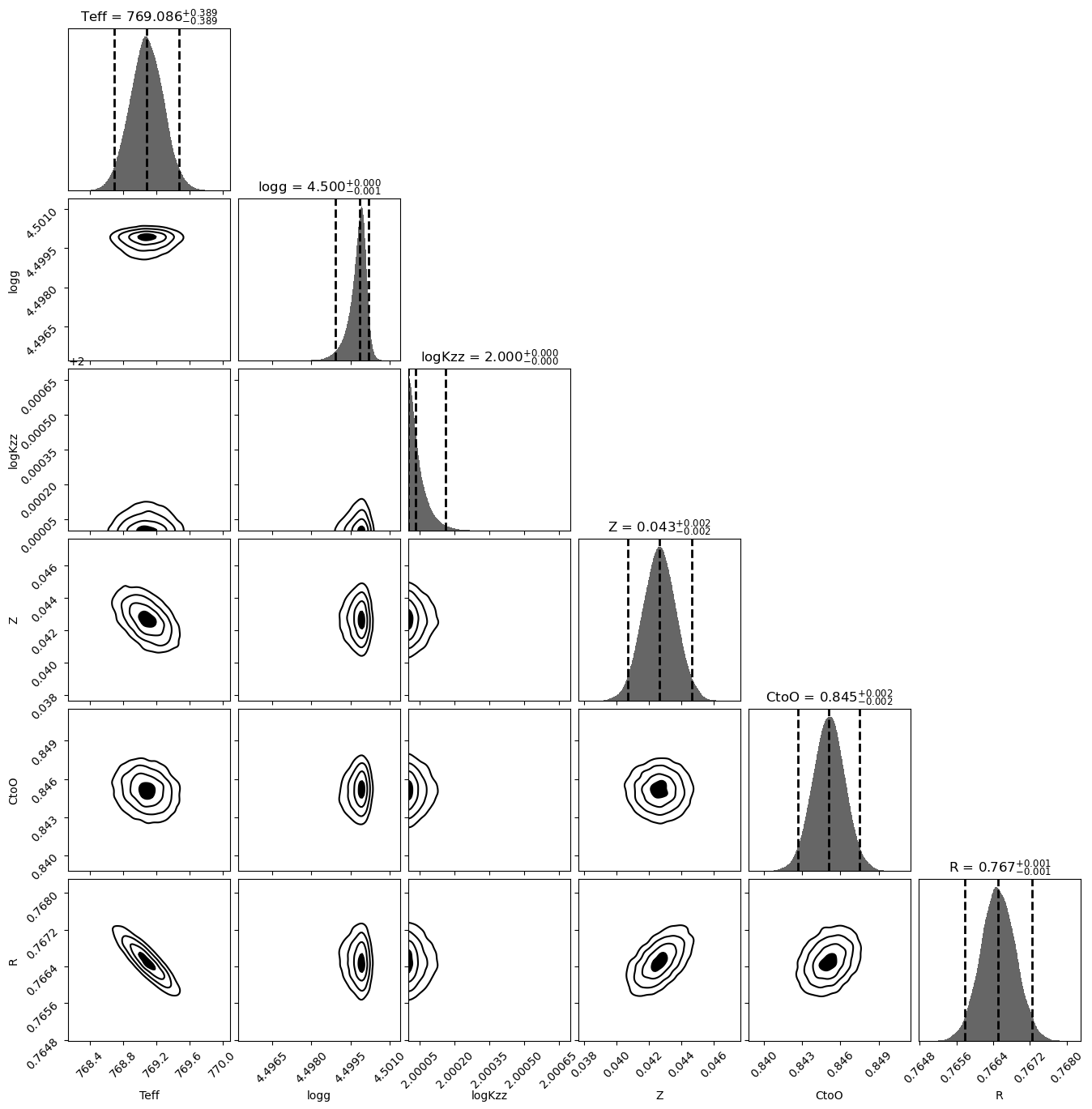
Make corner plot using dynesty tools:
[14]:
# plot the 2-D marginalized posteriors.
labels = list(out_bayes['my_bayes'].params_priors.keys())
fig, axes = dyplot.cornerplot(out_bayes['out_dynesty'], show_titles=True,
                              verbose='true', title_fmt='.3f',
                              title_kwargs={'y': 1.0}, labels=labels)
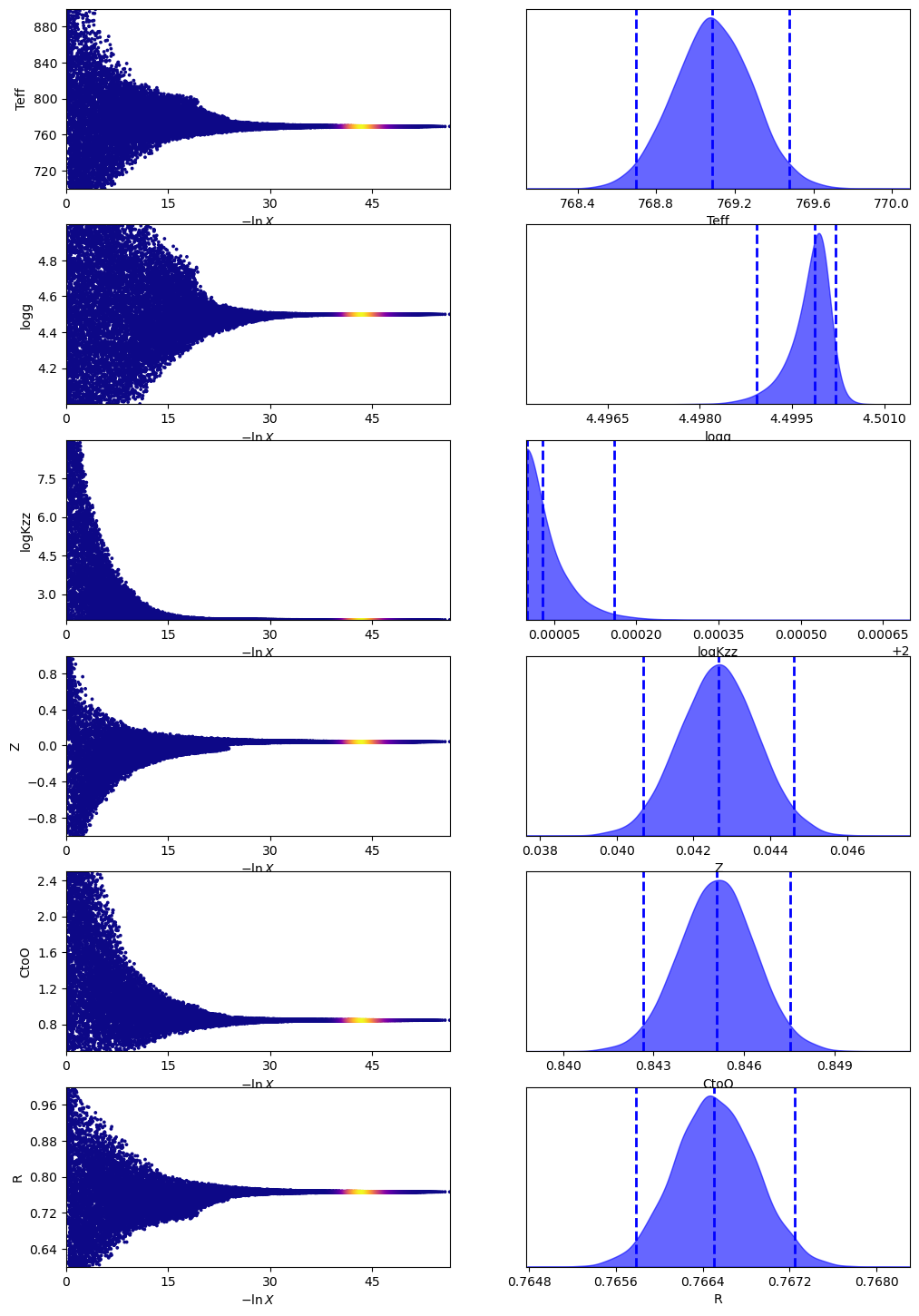
Quantiles:
Teff [(0.025, 768.6971245759519), (0.5, 769.0860309984688), (0.975, 769.4752476111898)]
Quantiles:
logg [(0.025, 4.498928972300711), (0.5, 4.499866635642559), (0.975, 4.500213413051319)]
Quantiles:
logKzz [(0.025, 2.0000010606607046), (0.5, 2.000030087030837), (0.975, 2.0001600380866966)]
Quantiles:
Z [(0.025, 0.04069622987874385), (0.5, 0.04265320251475469), (0.975, 0.04462163681636958)]
Quantiles:
CtoO [(0.025, 0.8426625773898881), (0.5, 0.8451112237279668), (0.975, 0.8475269129038827)]
Quantiles:
R [(0.025, 0.7657848929909543), (0.5, 0.766505990155875), (0.975, 0.7672444553747348)]
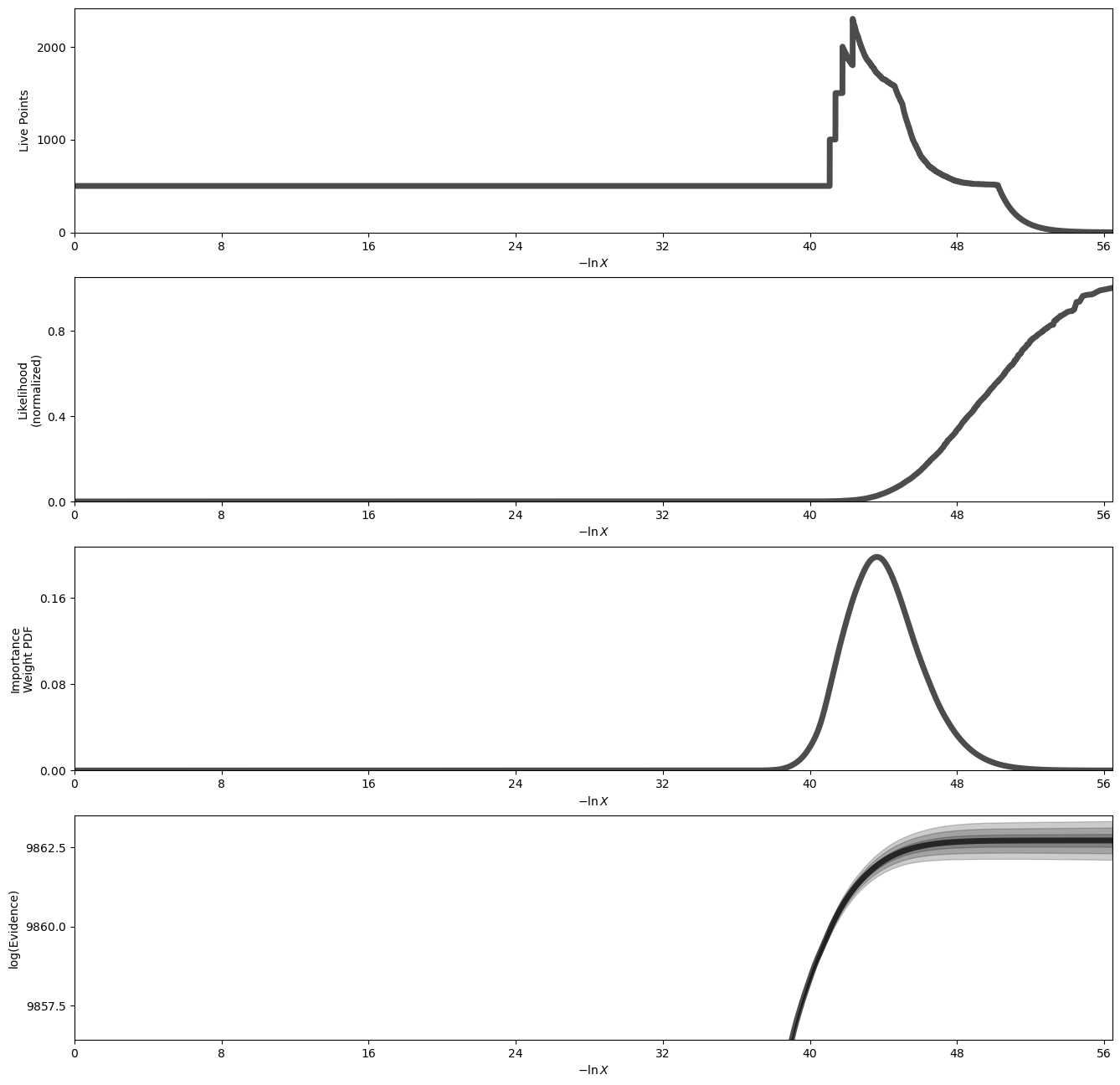
Plot a summary of the run
[15]:
fig, axes = dyplot.runplot(out_bayes['out_dynesty'], color='black',
                           mark_final_live=False, logplot=True)
Plot traces and 1-D marginalized posteriors
[16]:
fig, axes = dyplot.traceplot(out_bayes['out_dynesty'], labels=labels)
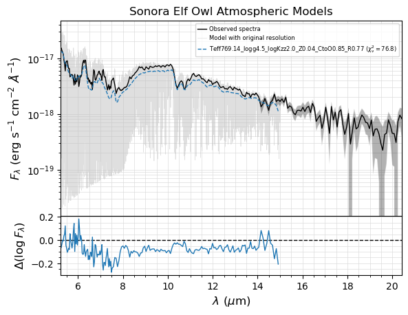
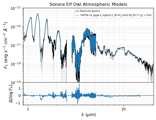
Plot the model spectrum using the median posterior parameters
SED with the best model fit from the Bayesian sampling.
The pickle file generated by seda.bayes_fit.bayes and stored with the name my_bayes.bayes_pickle_file is the input file to make plots. We can provide the name by either using my_bayes.bayes_pickle_file (if my_bayes is in memory) or just typing it.
The best model fit will be generated by interpolating into a model grid subset around the median posteriors.
Note that the Elf Owl models do not cover wavelenghts longer than 15 microns.
[8]:
# using default logarithmic scale for fluxes
fig, ax = seda.plots.plot_bayes_fit(bayes_pickle_file, xlog=True,
                                    yrange=[1e-19, 1e-15])#, ori_res=True)
For input spectrum 1 of 3

      8 model spectra selected with:
         Teff range = [750. 800.]
         logg range = [4.5 4.5]
         logKzz range = [2. 2.]
         Z range = [0.  0.5]
         CtoO range = [0.5 1. ]
      elapsed time: 1.0 s

For input spectrum 2 of 3

      8 model spectra selected with:
         Teff range = [750. 800.]
         logg range = [4.5 4.5]
         logKzz range = [2. 2.]
         Z range = [0.  0.5]
         CtoO range = [0.5 1. ]
      elapsed time: 0.0 s

For input spectrum 3 of 3

      8 model spectra selected with:
         Teff range = [750. 800.]
         logg range = [4.5 4.5]
         logKzz range = [2. 2.]
         Z range = [0.  0.5]
         CtoO range = [0.5 1. ]
elapsed time: 1.0 s
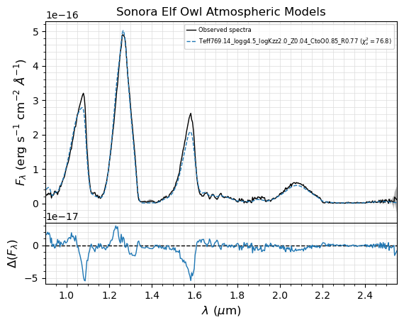
Zoom in on the SpeX spectrum:
[10]:
# plot fluxes in linear scale
fig, ax = seda.plots.plot_bayes_fit(bayes_pickle_file, ylog=False,
                                    xrange=[wl_SpeX.min(), wl_SpeX.max()])
For input spectrum 1 of 3

      8 model spectra selected with:
         Teff range = [750. 800.]
         logg range = [4.5 4.5]
         logKzz range = [2. 2.]
         Z range = [0.  0.5]
         CtoO range = [0.5 1. ]
      elapsed time: 1.0 s

For input spectrum 2 of 3

      8 model spectra selected with:
         Teff range = [750. 800.]
         logg range = [4.5 4.5]
         logKzz range = [2. 2.]
         Z range = [0.  0.5]
         CtoO range = [0.5 1. ]
      elapsed time: 0.0 s

For input spectrum 3 of 3

      8 model spectra selected with:
         Teff range = [750. 800.]
         logg range = [4.5 4.5]
         logKzz range = [2. 2.]
         Z range = [0.  0.5]
         CtoO range = [0.5 1. ]
elapsed time: 1.0 s
Zoom in on the NIRSpec spectrum:
[11]:
# plot fluxes in log scale
fig, ax = seda.plots.plot_bayes_fit(bayes_pickle_file,
                                    xrange=[wl_NIRSpec.min(), wl_NIRSpec.max()])
For input spectrum 1 of 3

      8 model spectra selected with:
         Teff range = [750. 800.]
         logg range = [4.5 4.5]
         logKzz range = [2. 2.]
         Z range = [0.  0.5]
         CtoO range = [0.5 1. ]
      elapsed time: 2.0 s

For input spectrum 2 of 3

      8 model spectra selected with:
         Teff range = [750. 800.]
         logg range = [4.5 4.5]
         logKzz range = [2. 2.]
         Z range = [0.  0.5]
         CtoO range = [0.5 1. ]
      elapsed time: 0.0 s

For input spectrum 3 of 3

      8 model spectra selected with:
         Teff range = [750. 800.]
         logg range = [4.5 4.5]
         logKzz range = [2. 2.]
         Z range = [0.  0.5]
         CtoO range = [0.5 1. ]
elapsed time: 1.0 s
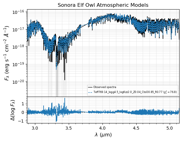
Zoom in on the IRS spectrum:
[12]:
# plot fluxes in log scale
fig, ax = seda.plots.plot_bayes_fit(bayes_pickle_file,
                                    xrange=[wl_IRS.min(), wl_IRS.max()],
                                    ori_res=True)
For input spectrum 1 of 3

      8 model spectra selected with:
         Teff range = [750. 800.]
         logg range = [4.5 4.5]
         logKzz range = [2. 2.]
         Z range = [0.  0.5]
         CtoO range = [0.5 1. ]
      elapsed time: 1.0 s

For input spectrum 2 of 3

      8 model spectra selected with:
         Teff range = [750. 800.]
         logg range = [4.5 4.5]
         logKzz range = [2. 2.]
         Z range = [0.  0.5]
         CtoO range = [0.5 1. ]
      elapsed time: 0.0 s

For input spectrum 3 of 3

      8 model spectra selected with:
         Teff range = [750. 800.]
         logg range = [4.5 4.5]
         logKzz range = [2. 2.]
         Z range = [0.  0.5]
         CtoO range = [0.5 1. ]
      elapsed time: 1.0 s

      7206 model spectra

      8 model spectra selected with:
         Teff range = [750. 800.]
         logg range = [4.5 4.5]
         logKzz range = [2. 2.]
         Z range = [0.  0.5]
         CtoO range = [0.5 1. ]
elapsed time: 0.0 s